For better or worse, most cell phones and digital cameras today can detect human faces, and, as seen in our previous post, it doesn’t take too much effort to get simple face detection code running on an Android phone (or any other platform), using OpenCV.
This is all thanks to the Viola-Jones algorithm for face detection, using Haar-based cascade classifiers. There is lots of information about this online, but a very nice explanation can be found on the OpenCV website.
 (image by Greg Borenstein, shared under a CC BY-NC-SA 2.0 license)
It’s basically a machine learning algorithm that uses a bunch of images of faces and non-faces to train a classifier that can later be used to detect faces in realtime.
The algorithm implemented in OpenCV can also be used to detect other things, as long as you have the right classifiers. My OpenCV distribution came with classifiers for eyes, upper body, hands, frontal face and profile face. While looking for information about how to train them, I found classifiers for bananas, pens and iPhones.
Actually, that last link is for more than just iPhones. In his Mirror Test project, Jeff Thompson is actually training computers to recognize themselves in a “non-utilitarian, flawed poetic/technological act”.
Similar to what we want, but since we have a very specific phone to detect, we decided to train our own classifier.
The OpenCV tutorial for Training Cascade Classifiers is a pretty good place to start. It explains the 2 binary utilities used in the process (opencv_createsamples and opencv_traincascade), and all of their command line arguments and options, but it doesn’t really give an example of a flow to follow, nor does it explain all the possible uses for the opencv_createsamples utility.
On the other hand, Naotoshi Seo’s tutorial is actually quite thorough and explains the 4 different uses for the opencv_createsamples utility. Thorsten Ball wrote a tutorial using Naotoshi Seo’s scripts to train a classifier to detect bananas, but it requires running some perl scripts and compiling some C++… too much work…
Jeff also has some nice notes about how he prepared his data, and a script for automatically iterating over a couple of options for the 2 utilities.
The way we did it was inspired by all of these tutorials, with some minor modifications and optimizations.
1. Negatives
This is where we gather about 1000 images of non-phones. Some people use video for this… we followed Jeff and took them from this repository, with this command:
cd negativeImageDirectory
wget -nd -r -A "neg-0*.jpg" \
http://haar.thiagohersan.com/haartraining/negatives/
Creating a collection file for these is pretty easy using the following command:
cd negativeImageDirectory
ls -l1 *.jpg > negatives.txt
2. Positives
This is where we gather about 1000 images of our phone. Some people use video, some people use scripts… we used scripts.
2a. Pictures
This is where we take pictures of our phone. We don’t need 1000 of them. Somewhere between 15 and 20 should be enough. This is what our images looked like:
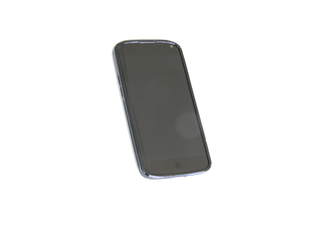
Since our object is pretty black, we used a white background, and took high-contrast pictures in order to make the next step easier. Also, the pictures don’t have to be large because OpenCV will shrink them anyway: ours were 1024x773.
2b. Process
This is where we use a Processing script to read the images and mark where the object is. Since we used high-contrast and a white background, it’s pretty easy to get an initial guess by just keeping track of the min/max x- and y- positions of dark pixels. What is important here is to make sure that the aspect ratio of all of the marked objects is the same. In our case, this was 1:1, and the script makes sure all the marked images follow that:
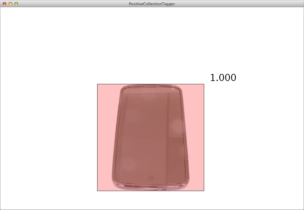
In addition to cropping the image, the Processing script also spits out a text file that has information about where the object is on the original image. This is what Naotoshi calls a description file format.
2c. Make 100s
This is where we venture away from Naotoshi. First, we run the following command for each of our cropped images:
opencv_createsamples -img cropped00.jpg \
-bg negativeImageDirectory/negatives.txt \
-info sampleImageDirectory/cropped00.txt \
-num 128 -maxxangle 0.0 -maxyangle 0.0 \
-maxzangle 0.3 -bgcolor 255 -bgthresh 8 \
-w 48 -h 48
Where cropped00.jpg is one of the cropped images from the Processing script, negatives.txt is the collection file for the negative images, cropped00.txt is where the opencv_createsamples utility will write its output description file.
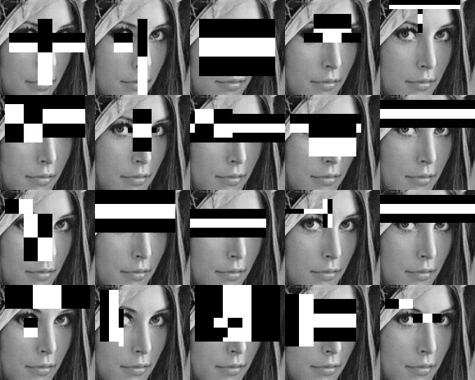
This will generate 128 images by placing a slightly rotated and slightly brighter/darker version of cropped00.jpg on top of a randomly selected negative image. And because we used a white background when we took our pictures, specifying 255 as the -bgcolor makes the white on the cropped image transparent, giving us 128 images like these:
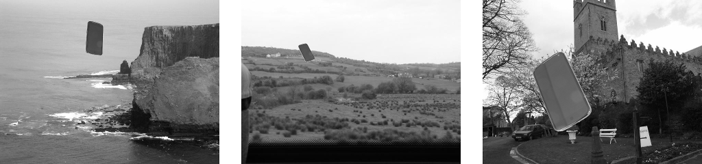
Running this command also generates a description file with information about where the cell phone is in each of the 128 images.
2d. Make 1000s
If we had 15 pictures, running the previous step on each of them would have produced 1920 pictures of cell phones floating in random places. What we have to do now is collect all of them into a single .vec file before we can run the training utility.
First, we collect all 15 description files into one, by running this command:
cd sampleImageDirectory
cat cropped*.txt > positives.txt
Then, we can combine all of them into a single .vec file using this command:
opencv_createsamples \
-info sampleImageDirectory/positives.txt \
-bg negativeImageDirectory/negatives.txt \
-vec cropped.vec \
-num 1920 -w 48 -h 48
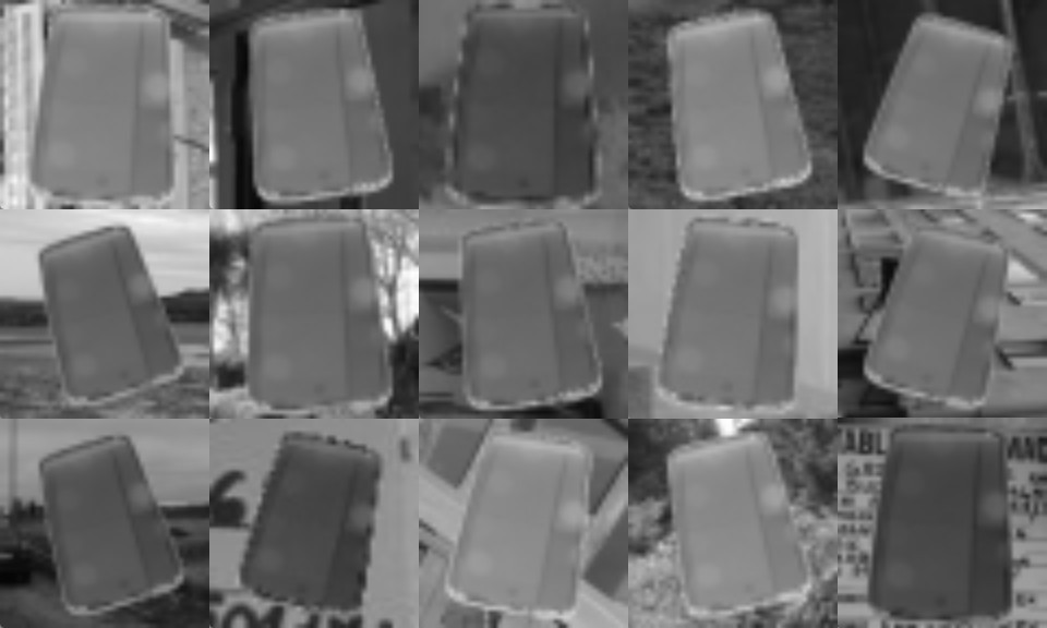
This will create 1920 cropped images of the cell phone, where each is rotated slightly different, and with a different background. Like this, but thousands:
3. Train the Cascade
This is where we train a Haar Cascade Classifier using another OpenCV utility. Armed with about 1000 negative images and 2000 positive images, we can run this command to start training:
opencv_traincascade -data outputDirectory \
-vec cropped.vec \
-bg negativeImageDirectory/negatives.txt \
-numPos 1000 -numNeg 600 -numStages 20 \
-precalcValBufSize 1024 -precalcIdxBufSize 1024 \
-featureType HAAR \
-minHitRate 0.995 -maxFalseAlarmRate 0.5 \
-w 48 -h 48
Most of these are the default values, one notable exception is the increase memory usage from 512Mb to 2Gb. Also, another thing to note, -numPos and -numNeg should be less than the total number of images actually available and described in the description/collection files. We found this out by trial and error, but it seems like the opencv_traincascade utility slowly increases the number of “consumed” images as it goes through the training stages, in order to meet the -minHitRate and -maxFalseAlarmRate, and when there are not enough images to consume, it crashes. For example, we specified -numPos 1000 for our runs, but by stage 10, it was “consuming” 1030 images.

If all goes well, a cascade.xml file should show up in the outputDirectory after a couple of hours (or days).
We wrote a script that automates most of this process.
With these settings, it took our training about 24 hours to complete. While waiting for the 20 stages to finish, the same opencv_traincascade command can be run in parallel to create a partial cascade file from the stages that are already complete. For example, the following command will generate a cascade from the first 10 stages of classifiers in the output directory:
opencv_traincascade -data outputDirectory \
-vec cropped.vec \
-bg negativeImageDirectory/negatives.txt \
-numPos 1000 -numNeg 600 -numStages 10 \
-precalcValBufSize 1024 -precalcIdxBufSize 1024 \
-featureType HAAR \
-minHitRate 0.995 -maxFalseAlarmRate 0.5 \
-w 48 -h 48
It’s basically the same command, but with -numStages set to 10.
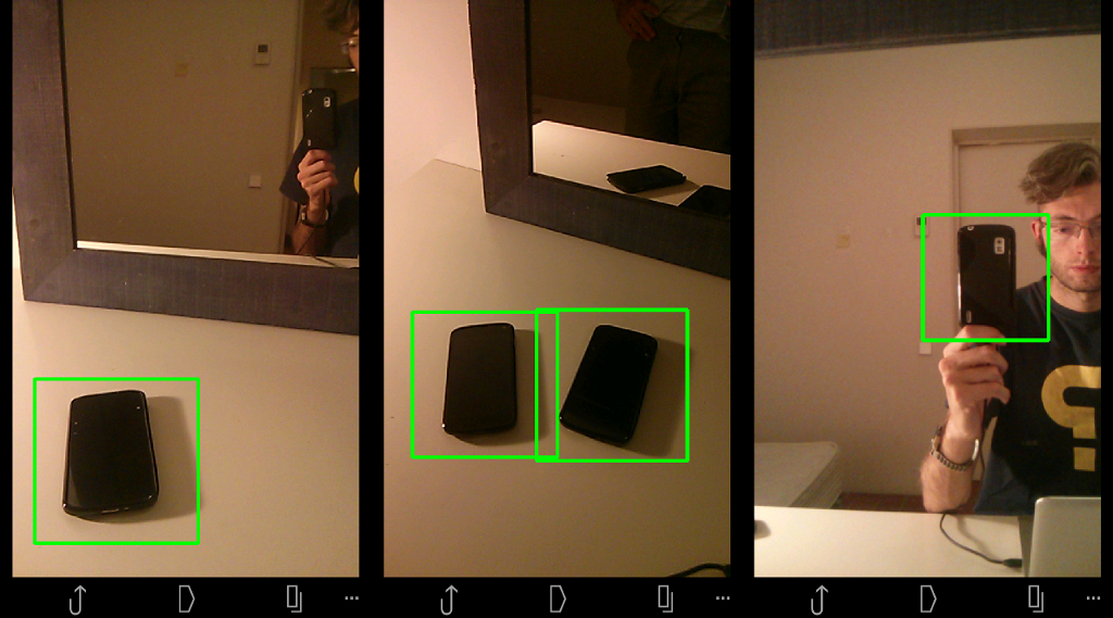
Some initial tests on a laptop computer, using ofxCv:
Nice !!!
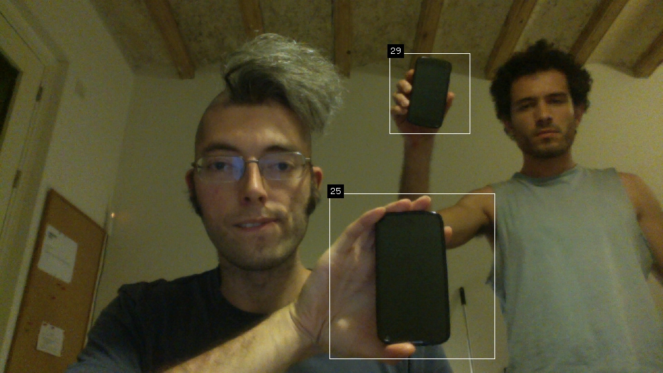
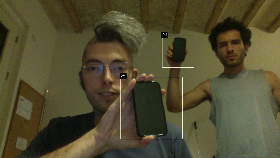
Some tests running on an Android phone:
Hooray !!! It recognizes itself and its friends !!!